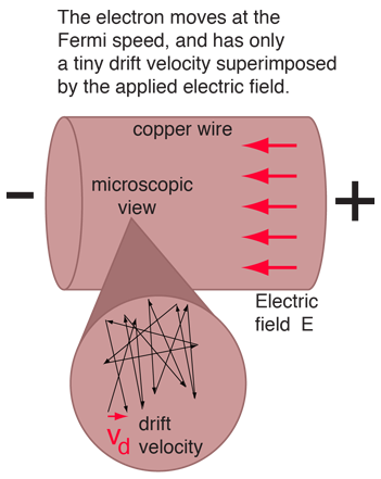
Microscopic View of Copper Wire
As an example of the microscopic view of Ohm's law, the parameters for copper will be examined. With one free electron per atom in its metallic state, the electron density of copper can be calculated from its bulk density and its atomic mass.

The Fermi energy for copper is about 7 eV, so the Fermi speed is

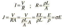
The measured conductivity of copper at 20°C is

The mean free path of an electron in copper under these conditions can be calculated from

The drift speed depends upon the electric field applied. For example, a copper wire of diameter 1mm and length 1 meter which has one volt applied to it yields the following results.

For 1 volt applied this gives a current of 46.3 Amperes and a current density

This corresponds to a drift speed of only millimeters per second, in contrast to the high Fermi speed of the electrons.

Caution! Do not try this at home! Dr. Beihai Ma of Argonne National Laboratory wrote to point out that the current density of 5900 A/cm2 in this example is over ten times the current density of 500 A/cm2 that copper can normally withstand at 40°F. So doing this in the laboratory might be too exciting. Thanks for the sanity check Dr. Ma.
(If you scale down the voltage applied so that the current is just 3 Amperes, current density 382 A/cm2, so that the copper wire will remain intact, the calculated drift velocity is just 0.00028 m/s. This would be more typical for working conditions in this wire. )
What about quantum effects and Fermi-Dirac statistics?
The treatment of the microscopic Ohm's Law and drift velocity above is basically a classical treatment. But we know that the electrons in a metal obey Fermi-Dirac statistics, and that at low temperatures, all the available electron energy levels are filled up to the Fermi Level. We also know that this Fermi level (about 7 eV in copper) is very high compared to room temperature thermal energy. Then how do we justify using the whole free electron population above in the calculation of drift velocity when for thermal interactions, only those electrons within about kT of the Fermi Level are accessible to the interaction?
One place where this situation is discussed is in the classic Solid State Physics book by Charles Kittel. He points out that because of the full population of conduction electrons up to the Fermi level, these electrons in the copper wire have a very high velocity, on the order of 1.6 x 106 cm/sec for copper. An externally applied electric field in a copper wire will exert a continuous force on the electrons and would continue to accelerate them if that acceleration were not randomized by the multiple collisions and interaction with the lattice. The observation of Ohm's Law experimentally shows us that an equilibrium current is achieved, and that the presumption that all the conduction electrons are participating allows us to project an effective drift velocity for these electrons under the influence of the applied electric field. It is noted that this is an entirely classical presumption.
As Kittel further examines electrical conductivity from the point of view of Fermi-Dirac statistics, he makes the following comment: "It is a somewhat surprising fact that the introduction of the Fermi-Dirac distribution in place of the classical Maxwell-Boltzmann distribution usually has little influence on the electrical conductivity, often only changing the kind of average used in the specification of the relaxation time. One might have expected at first sight to find a more drastic change because with the Fermi-Dirac distribution only those electrons near the Fermi surface can participate in collision processes. "
Kittel argues that the exclusion principle does not prevent the electric field intervention since it acts on each electron in the distribution to produce the same velocity change. There is always a vacant state ready to receive the electron which is changing its state under the action of the electric field, the vacancy being produced by the simultaneous change of the state of another electron. In contrast to a random thermal collision process, the single direction electric force produces electron excess states A and electron deficiency states B which allow the specific collisions required to restore equilibrium. The exclusion principle does prevent many collisions, but does allow those collisions needed to restore equilibrium. The bottom line is, except for the detailed nature of the relaxation time, the situation is essentially the same as in the classical situation, and leads to the same conductivity expression and average drift velocity.
|