Motion Graphs

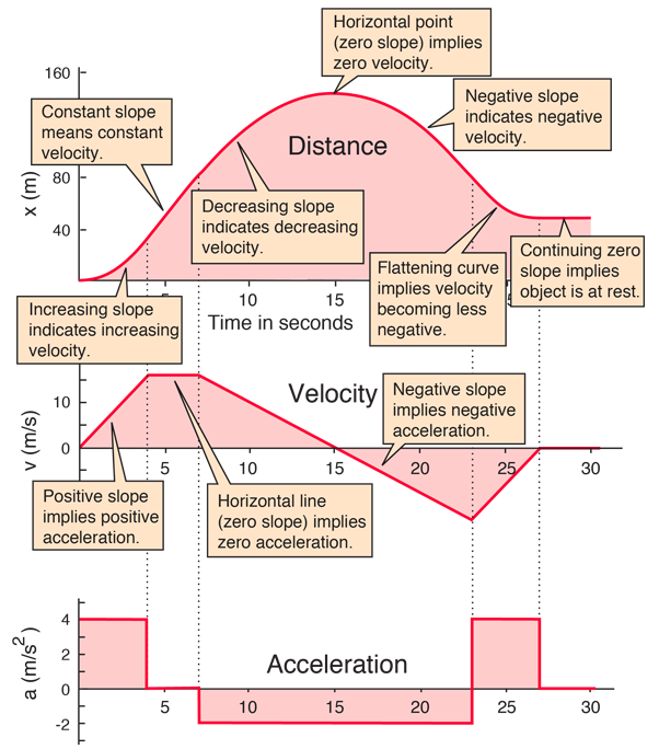
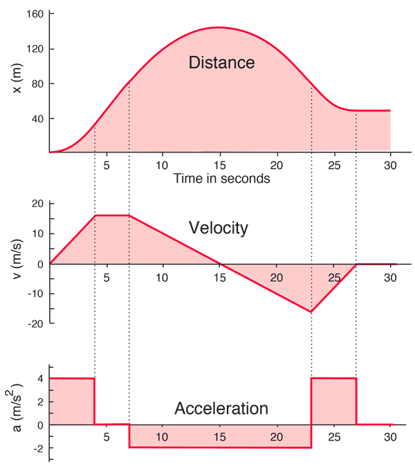
Constant acceleration motion can be characterized by motion equations and by motion graphs. The graphs of distance, velocity and acceleration as functions of time below were calculated for one-dimensional motion using the motion equations in a spreadsheet. The acceleration does change, but it is constant within a given time segment so that the constant acceleration equations can be used. For variable acceleration (i.e., continuously changing), then calculus methods must be used to calculate the motion graphs.

Add annotation about the slopes of the graphs.

A considerable amount of information about the motion can be obtained by examining the slope of the various graphs. The slope of the graph of position as a function of time is equal to the velocity at that time, and the slope of the graph of velocity as a function of time is equal to the acceleration.

Index

Motion concepts
 
HyperPhysics***** Mechanics R Nave
Go Back


The Slopes of Motion Graphs

A considerable amount of information about the motion can be obtained by examining the slope of the various motion graphs. The slope of the graph of position as a function of time is equal to the velocity at that time, and the slope of the graph of velocity as a function of time is equal to the acceleration.

In this example where the initial position and velocity were zero, the height of the position curve is a measure of the area under the velocity curve. The height of the position curve will increase so long as the velocity is constant. As the velocity becomes negative, the position curve drops as the net positive area under the velocity curve decreases. Likewise the height of the velocity curve is a measure of the area under the acceleration curve. The fact that the final velocity is zero is an indication that the positive and negative contributions were equal.

Index

Motion concepts

Velocity and acceleration
 
HyperPhysics***** Mechanics R Nave
Go Back