Cavity Resonance
The purpose of this experiment is to explore the resonant behavior of acoustic cavities (a coke bottle and your voice). Recall that a resonant frequency is defined as a natural frequency of vibration which is determined by the physical properties of the vibrating object. In this case the physical properties which affect the natural frequency of the cavity are its volume, area of opening, and length of opening port. In this experiment, only the effects of changing volume will be explored since the other factors are not easily changed.
The apparatus consists of a coke bottle, a graduated cylinder, and a digital computer interface with which to produce a digital image of the sound made by blowing over the coke bottle. The computer interface can also be used to collect data on your voice.
Procedure: Setup of Computer Interface:
1. Double-click on the DataStudio icon to start the data collection software.
2. Scroll down the "Sensors" menu to "Sound Sensor" and click-and-drag t hat icon to the image of the port where your microphone is connected.
Data Collection:
1. Click on "Scope" under the "Displays" menu to display an oscilloscope screen. Click the "Start" button and produce a sound to confirm that you can display a sound waveform. You may need to adjust the V/div(sensitivity) and/or Offset (vertical position) controls until get a satisfactory waveform with no clipping of the peaks. Experiment with starting and stopping the display.
2. Click the "Start" button and blow over the coke bottle close to the microphone, but do not blow directly on the microphone. Once you are producing a satisfactory waveform, click the "Stop" button to hold the display. You can repeat this part if you like to get a better waveform.
3. Click the data storage button to store that trace of the sound waveform. This button looks like pincers picking up a ball. Then double-click on "Graph" under the "Displays" menu to put a graph on the screen. Drag the icon for your data set over onto the graph to display it. It will appear cluttered with their cute symbols for data points, but you can clean it up by going to the Display/Settings and taking off the "Show data points" and "Show Legend Symbol" options.
4. Measure the time associated with the first clear peak on the waveform. Then move the cursor to the last clear peak to the right and record that time as "End Time". You can just read the numbers off the graph, or go Display/Measure to display a set of crosshairs on the screen to make measurements. Try both ways to see which you like best. Record the number of periods spanned and calculate the period and frequency of the wave.
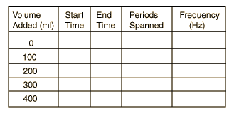
5. Repeat the process after adding 50 ml (same as cm3) of water from a graduated cylinder. Repeat for added volume 100, 150 and 200 ml.
6. Plot your data with frequency in Hz on the vertical axis and the added volume on the horizontal axis.
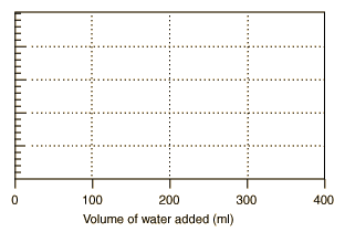
Prediction-verification:
7. From your graph, predict the frequency which should be produced if 125 cm3 is added to the empty bottle. Then measure that frequency by the procedure outlined above for comparison.
Predicted frequency for 125 cm3 added _________.
Measured frequency _________
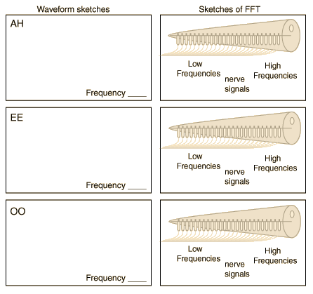
8. Now record your voice for three vowel sounds, "AH" as in "father", "EE" as in "heed", and "OO" as in "who". As you record each, sketch the waveform in the space provided and determine the frequency. Then click on the FFT option and drag it onto the work area and display the FFT (Fast Fourier Transform) of the sound. It gives you the intensity as a function of frequency. Do a rough sketch of that FFT on the sketch of the inner ear's basilar membrane to represent how that frequency pattern would be detected by the inner ear. The point is to see how different the patterns are and to give some impression of how the human ear distinguishes these sounds.